David A. Kenny
September 11, 2011

Being revised after 12 years.

Please send comments and suggestions.

Respecification of Latent Variable Models

**These simplifications in the model do not usually improve the model's fit and are in purple.

Those in black without asterisks may improve the fit of the model.

Step A:  Is the measurement model consistent with the data (i.e., good fitting)?

Yes, go to Step C.
No, go to Step B unless you have exhausted reasonable respecifications.  IF SO, THEN  STOP!

Step B:  Revise the measurement model.  (Go to the CFA page for other ideas.)

          Strategies for respecification

correlation matrix

modification index (Lagrangian multiplier in EQS)

definition: The approximate increase in chi square if the parameter were free

                             zero implies parameter

                                      already estimated

                                      not identified

                                      estimated as zero

sequence: a large modification index may be explained by some other specification error

Some modification indices (especially with Amos) may be implausible and should be ignored

standardized residual: Difference between predicted and observed covariance standardized

          What to respecify?

Factor loadings

Too small?  Drop the measure?**
Too large, Heywood cases?**
        possible specification error
        constrain error variance to be non-negative
Set the loadings equal?  (Measures should have the same metric and the covariance matrix analyzed.) **

Error variances

Too small or negative: Heywood cases?**
Set the error variances equal?  (Measures should have the same metric and the covariance matrix analyzed.) **

Need fewer factors?

Poor discriminant validity?  (Combine factors.)**
Make sure each factor has sufficient variance.  (Drop factors)**

Need more factors?

Run a maximum likelihood exploratory factor analysis to test the number of factors (see how to do this).  (Note that this test presumes no correlated errors and so might be misleading if the true model has correlated errors.)

Evaluate measures

Check to see if a measure has large standardized residuals and modification indices (Lagrangian multipliers in EQS).  Consider dropping that measure.

Need correlated errors?

Considerations

Meaningfulness Rule:  Only correlate errors for which there is a theoretical rationale.

Transitivity Rule:  If X₁ is correlated with X₂ and X₂ with X₃, then X₁ should be correlated with X₃ unless one pair is correlated for one reason and the other for a different reason.

Generality Rule:  If there is a reason for correlating the errors between one pair of errors, then all pairs for which that reason applies should also be correlated.

Sometimes correlated errors imply an additional factor.  For example, if X₁, X₂ and X₃ all have correlated errors, then consideration might be given to adding a factor on which the three load.

Single indicator variables may not have correlated errors but indicators of other factors may load on the single indicator "factor."

Which errors to correlate?

large modification indices

large standardized residuals

Need measures to load on more than one factor?  (Read about identification difficulties.)

When done return to Step A.

Step C:  If the structural model is just-identified go directly to Step D.

        Are the deleted paths in the structural model actually zero?

                  No, go to Step D.

Yes, add in deleted paths (see how deleted paths are defined) and go to Step D.

Step D:  Are the specified paths of the structural model needed?

Yes, keep in model.
No, consider trimming from model.**

Equivalent Models

Even if one's model fits, there are a myriad of other models that fit as  well.  These equivalent models should be considered.  Realize that for any model, there always exist an infinite number of models that fit exactly the same.  Thus, although the fit of the structural model confirms it, it in no way proves it to be uniquely valid.

Respecification Strategies

There are two strategies to take in the process of re-specifying a model.  One can test a priori, theoretically meaningful complications and simplifications of the model.  Alternatively, one can use empirical tests (e.g., modification indices and standardized residuals) to respecify the model.  All respecifications should be theoretically meaningful and ideally a priori.  Too many empirically based respecifications likely lead to capitalization on chance and over-fitting (unnecessary parameters added to the model).  Ideally, if many respecifications are made, a replication of the model should be undertaken.  Although a priori hypotheses deserve the initial focus, an examination of empirical tests of miss-specification are in order.  But if model changes are made on the basis of such tests, there still need to be some sort of theoretical rationale for them.

Example

          Consider the following study: Reisenzein, R. (1986).  A structural equation analysis of Weiner's attribution-affect model of helping behavior.  Journal of Personality and Social Psychology, 50, 1123-1133.

The study asks UCLA students to imagine that they are on a subway and they see a man lying on the ground and he appears to blind (a white cane is next to him) or drunk (an empty whiskey bottle is next do him).  Do you help this man?

Measurement Model

Control                                    Anger

          C₁: controllable                    A₁: anger

          C₂: responsible                    A₂: irritated

          C₃: fault                                A₃: aggravated

Sympathy                              Helping

          S₁: sympathy                       H₁: likelihood of helping

          S₂: pity                                 H₂: certainty

          S₃: concern                         H₃: amount

Scenario:

single indicator dichotomy, no measurement error, experimentally manipulated; 0 = blind and 1 = drunk                       

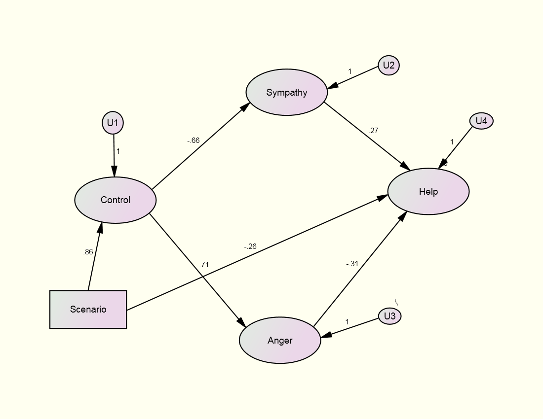
Structural Model

Control = Scenario + U1

          Anger = Control + U3

          Sympathy = Control + U2 

(disturbances of U2 and U3 correlated)

          Helping = Anger + Sympathy + U4

Specified Model

The fit of the specified model is

χ²(60) = 87.507 p = .012 (fit: TLI = .974 and RMSEA = .058)

Most investigators would stop here.  We adopt a different approach.

Note the df of the measurement is 56 and the df of the structural model is 4, making the total df 60.

Respecification of the Reisenzein Model

Step A: Fit of the Measurement Model or Just-identified Structural Model

          χ²(56) = 81.63, p = .014 (TLI = .974; RMSEA = .058)

The fit is good, but it might be improved. 

Step B: Revised Measurement Model

Let us examine at the largest modification indices:

Covariances:                      M.I.    Par Change

  E9 <-------------> Help         16.103       0.154

Regression Weights:           M.I.    Par Change

   S3 <------------- Help         10.581       0.198

   S3 <---------------- H3         11.564       0.188

   S3 <---------------- H1         11.500       0.187

The modification indices point to the S3 (concern) loading on the Help factor.  Because this makes sense, the measurement model is revised allowing for this loading.  (One might argue that S3 should be dropped as it is not a clean indicator.)

Test Revised Measurement Model

χ²(55) = 58.89, p = .335 (TLI = .996; RMSEA = .023 and 0 is in the 90% confidence interval)

There are no Heywood cases and all of factor correlations (except between Scenario and Control) are less than .85.  The fit of the measurement model is deemed acceptable.  We can live with this large correlation because it is in essence a manipulation check.

Step C: Test of the Deleted Paths (paths assumed to be zero)

The tests of the deleted paths are as follows:

Cause        Effect         Beta  Z-Value

Scenario    Anger          .052  0.327

Scenario    Sympathy .126  0.767

Scenario    Helping     -.354 -2.340

Control      Helping       .186  0.836

So the only deleted path needed is the path from Scenario to Helping.  The path is negative indicating a willingness to help the control person, the blind man, than the drunk man.  The combined test of the four deleted paths is χ²(4) = 8.07, p < .10.

Step D: Test of the Specified Paths and Correlation

All of the specified paths are statistically significant.  However, the correlation between the disturbances of Anger and Sympathy is not statistically significant (Z = 1.213).

Step E: Trimmed Model

The correlation between the disturbances of Anger and Sympathy is set to zero.

Factor Loadings

Control       .74
Sympathy      .43
Anger         .50
Help          .50